 ARCTIC SYSTEMS
TECHNICAL DOCUMENTATION / VERIFICATION
Results, with their conditions.
Independent analytical references and manufactured solutions test the numerical implementation. They do not establish agreement with a real site.
Start with the 1D reference; compare methods of locating the front. Then explore 2D boundaries and 3D convergence. Open the setup below each graph for the full assumptions.
A sharp-front reference
ANALYTICAL · NEUMANN / STEFAN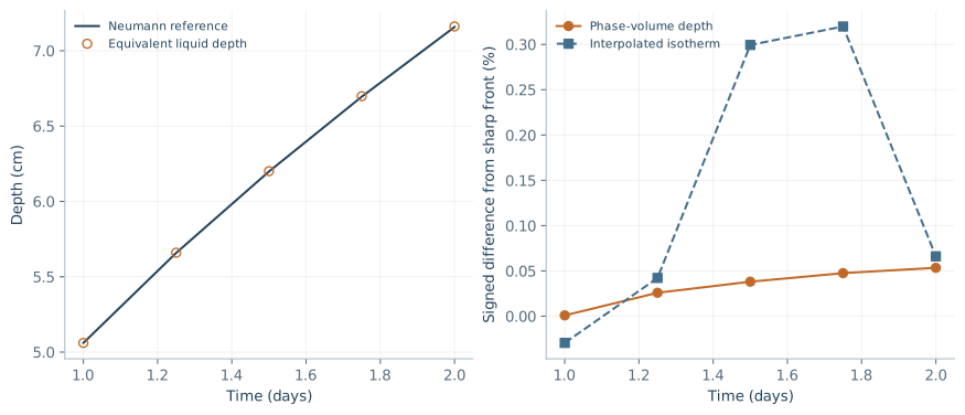
Selected refined result
At day 2: RMS temperature error 0.002579 K; maximum temperature error 0.008545 K; equivalent liquid-depth difference +0.05345%.
These are different observables. An integral phase volume represents a front position only in the limit of one sharp monotone interface. It is not generally an isotherm.
Why the right-hand curves separate
The right axis is percent error, not temperature. Both curves describe the same run: blue locates an interpolated isotherm; orange converts the liquid-phase volume into an equivalent depth.
At day 1.75 the blue difference is 0.32% ≈ 0.21 mm at a reference depth of about 67 mm. The cell width is 0.625 mm. The orange difference there is about 0.032 mm. The vertical scale magnifies small differences; 0.32% does not mean 32%.
The regularized transition moves relative to the cell centres, making the isotherm observer sensitive to its position. Space, time and regularization errors remain; a small fraction of a cell is not by itself an acceptance criterion.
Refining only the mesh at fixed transition width did not reduce every error monotonically. The displayed fine case controls mesh, time and transition width together.
Earlier coarse-grid diagnostic: a different case
The historical 4.65% isotherm error belongs to a 200-cell case with 0.05 K transition width, not the 3200-cell curve above. The same observer applied to projected exact enthalpy gave 4.60% without solving the PDE, isolating a large observer bias in that coarse case. It does not assign all error in the refined case to interpolation.
Full selected setup, reference and interpretation
Melting in a homogeneous half-space: surface +10°C, far field −4°C, melting temperature 0°C. Frozen/thawed k = 2/0.6 W/(m·K); sensible C = 2/4 MJ/(m³·K); Lv = 334 MJ/m³. These are synthetic test properties, not a measured soil.
s(t) = 2λ√(αneart), λ = 0.2222815969248, obtained from the classical interfacial energy balance. The independent reference uses error-function temperature profiles. The computed interval 0–2 m uses the exact solution at both boundaries; initial cell enthalpies are volume-averaged from the reference at day 1.
Selected case: 3200 cells, Δx = 0.000625 m, Δt = 56.25 s, transition width 0.0125 K, days 1–2. No singular t = 0 start. Five saved times are shown. Different refinement factors were studied separately in the archived 16-case diagnostic. Reference formulation.
Phase change with mixed boundaries
2D · MANUFACTURED SOLUTION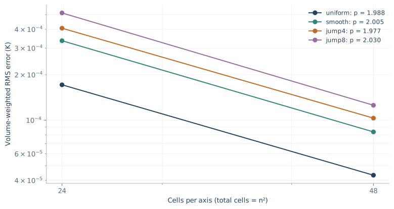
Controlled spatial refinement
36 primary runs and 8 time-control runs. The last spatial orders are 1.977–2.030 for these temperature fields. RMS is weighted by actual cell volumes.
The graph uses 2T(Δt/2) − T(Δt) to reduce the leading time error. These are diagnostic extrapolated fields, not the ordinary output of a single solver run.
| Mesh | Order p | Residual ratio* |
|---|---|---|
| uniform | 1.9878 | 7.67% |
| smooth | 2.0048 | 4.07% |
| jump4 | 1.9770 | 3.23% |
| jump8 | 2.0300 | 2.78% |
*Change between successive time extrapolations / fine extrapolated RMS. This is not a rigorous error bound. The raw fine-grid RMS at Δt = 0.0005 s is about 0.000146–0.000153 K.
Exact field, material, mesh and boundary conditions
T = −0.1 + 0.23 sin(2πt) cos[π(x + 0.137)/1] cos[π(z + 0.211)/1.3]. Coordinates are in m and time in s; the trigonometric factors use these stated scales. Domain 1 × 1.3 m, unit extrusion; t = 0.05 to 0.35 s. Cf/Ct = 2/3 J/(m³·K), kf/kt = 1/1.8 W/(m·K), Lv = 8 J/m³, phase interval −0.2 to 0°C. Synthetic scales, not soil parameters.
Q = CappTt − k∇²T − k′|∇T|² is derived independently. Exact initial temperatures at cell centres; left/top Dirichlet; bottom exact outward Neumann; right Robin h = 7 W/(m²·K), with Tambient = T + kTx/h. Ambient is manufactured for this test, not weather.
Static uniform, smooth and abrupt 4:1 / 8:1 grids. Primary n = 12, 24, 48 with Δt = 0.004, 0.002, 0.001 s; extra Δt = 0.0005 s at n = 24, 48. The plotted final diagnostic uses 2T(0.0005) − T(0.001). A quadratic-field audit separately shows first-order local flux error at abrupt mesh-size jumps. No claim of arbitrary-grid second-order accuracy.
A genuinely three-dimensional phase field
3D · MANUFACTURED SOLUTION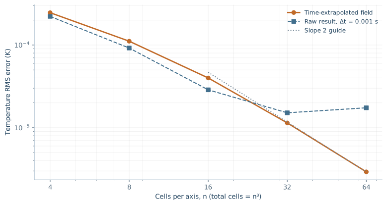
What has been demonstrated
The final spatial diagnostic order is 1.966 on 32³ → 64³. This is a field varying along all three axes and in time, with nonlinear phase heat capacity.
The raw curve is shown too: at fixed Δt, refining space can expose temporal error and cancellation. The smaller extrapolated errors are not substituted for raw solver accuracy.
| Mesh | Raw Δt .001 | Extrapolated | p |
|---|---|---|---|
| 4³ | 0.00022205 | 0.00024603 | — |
| 8³ | 9.1979e-05 | 0.00011122 | 1.145 |
| 16³ | 2.8715e-05 | 3.9949e-05 | 1.477 |
| 32³ | 1.514e-05 | 1.1424e-05 | 1.806 |
| 64³ | 1.7408e-05 | 2.9238e-06 | 1.966 |
Setup, time control and linear-solver qualification
T = −0.1 + 0.07 sin(2πt) ∏acos(πxa/La), L = (1, 1.3, 0.7) m; t = 0.05 → 0.13 s. The time factor uses seconds. All six boundaries and initial cell temperatures use the exact field; the source is its independently differentiated energy balance. Cf/Ct = 2/3 J/(m³·K), kf/kt = 1/1.8 W/(m·K), Lv = 8 J/m³, phase interval −0.2 to 0°C.
The spatial diagnostic combines Δt = 0.002 and 0.001 s. An additional Δt = 0.0005 s on 32³ changes the extrapolated field by RMS 5.886 × 10⁻⁸ K, or 0.513% of the finer extrapolated error. That third time level was not run on 64³; no rigorous residual bound is claimed there.
Large diagnostic runs used a scaled BiCGSTAB/Jacobi linear solve, checked against the direct solve at 16³: maximum difference 3.581 × 10⁻¹² K. The production workbench retains its direct sparse solve. Early linear-solver failures and a timed-out 64³ attempt remain archived; the selected final run completed separately. This is not a web capacity benchmark.
View three slices of the saved 3D result
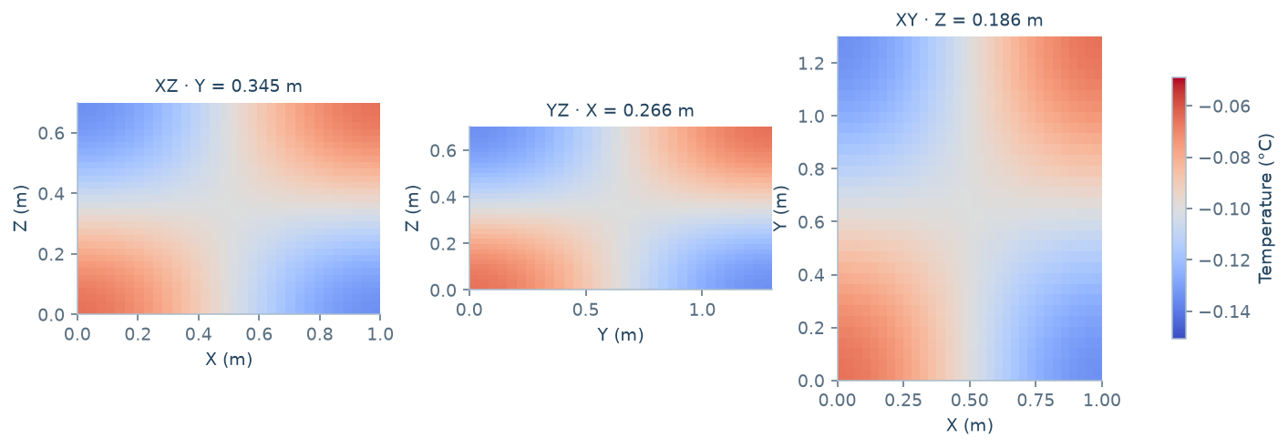
32³, Δt = 0.001 s, t = 0.13 s; cell planes near one-quarter of each axis with their exact coordinates. Shared scale. Raw saved field, not extrapolated. This is also an alternative illustration to the building.
Two heat inputs, one initially frozen ground
SYNTHETIC · EDUCATIONAL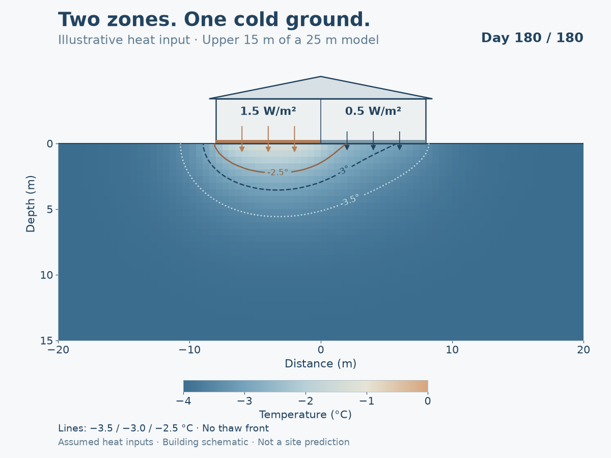
The setup
Domain 40 × 25 m, unit extrusion. Initially −4°C; k = 2 W/(m·K), C = 2 MJ/(m³·K). The top receives inward 1.5 W/m² over x = −8…0 m and 0.5 W/m² over x = 0…8 m; the rest is insulated. Sides and bottom stay at −4°C.
Selected mesh 80 × 50, Δt = 0.5 day, duration 180 days. The image displays only the upper 15 m of the computed 25 m. The building is a drawing, not a simulated room or structural model.
Maximum cell temperature is about −1.343°C. The phase interval is never entered. All three contours represent warming within frozen ground, not a thaw front.
What was checked
Six saved runs varied mesh, time and domain. Maximum differences at common temperature probes decreased from 0.02560 to 0.01276 K under successive mesh refinement, and from 0.00674 to 0.00373 K under successive time refinement. The expanded-domain difference was 0.00600 K. These are differences between runs, not true-error bounds.
The heat inputs are assumed illustration parameters, not established losses from occupied rooms. Contour appearance at early times remains sensitive; display starts at the documented later times.